Image/point cloud alignment based on depth information
Things get easier when depth information is available.
These days I was trying to align multiple images obtained by a custom stereo camera. In the beginning, I thought I could just utilize the conventional method, such as matching the feature points between two consecutive images. Since it is a stereo camera, depth information is right at my disposal, things seem so straightforward. At first, we thought it might not work since we are taking pictures of low texture and random texture objectives. It might be difficult to match the feature points. After a painful tuning process, it finally worked.
The left image of the custom stereo camera is taken as the base image. The depth is calculated with respect to the left image. The camera is under constant movement, we will use the left images at different camera poses to try to get an alignment. After aligning the images, point clouds, which are obtained by reprojecting depth information into 3D space, are aligned in MeshLab.
Thanks to OpenCV, it has everything we need to accomplish this task.
The procedures are as follows:
- Perform stereo reconstruction at the new camera location. Reproject the depth information to 3D space forming point cloud.
- Take the left images of the current and previous camera location. Compute and match the feature points in those images.
- Calculate the relative camera pose between the two camera locations.
- Repeat the above processes until all the camera locations are processed.
- Compose MeshLab project file, importing the point clouds and align them with each other.
Following the instructions of OpenCV, I was using SURF feature points and the FANN matcher. Let’s define the left image of the previous location as Image 0 and Image 1 for the new camera location. The depths are found for the matched feature points in Image 1. Then the 3D coordinates of these feature points are calculated. At this moment, we have the 2D feature points in Image 0, and their corresponding 3D counterparts defined in the reference frame of Image 1. We could use SolvePnPRansac() to compute the relative camera pose of Image 1 with respect to Image 0. Once the relative pose is obtained, we could take Image 1 as Image 0 and repeat the above process with the next camera location. The location of the very first stereo image pair is taken as the global origin. Successive camera locations are calculated with respect to this origin. After all the camera locations are obtained, a MeshLab project file is composed. In this MeshLab project file, each point cloud is associated with a transformation based on their left camera poses. MeshLab reads the project file and imports all the point cloud and aligns them together automatically.
Thera are actually some points that I would like to share.
The most important one is that as we are taking advantage of the stereo camera, which gives us depth information of an image, the images have been through rectification. For a stereo to work properly, one needs to perform stereo calibration on the stereo camera and the images are rectified based on the calibration. After rectification, the rectified images are utilized to do a stereo reconstruction to get the depth. The depth is directly associated with the rectified image but not the original, un-rectified image. As mentioned, the rectification uses the results of the stereo calibration rather than the calibration performed on a single camera. That means one should be very careful about the input arguments of initUndistortRectifyMap() while performing image rectification.
After the point clouds get aligned in MeshLab, people may want to project the left images onto those point clouds as textures. The key is to align the 2D raster images to the transformed point clouds. In MeshLab, the 2D rasters are transformed “inversely” with respect to the point clouds. To be specific, in the MeshLab project file, the rotation and translation for element <MLMatrix44> and element <VCGCamera> are “inverse” with each other. By inverse, I mean if you put a rotation matrix \(\left [ \mathbf{R} \right ]\) and a translation vector \(\left \{ \mathbf{T} \right \}\) directly into the matrix under element <MLMatrix44>, you will need to put \(\left [ \mathbf{R}^{\mathrm{T}} \right ]\) and \(− \left [ \mathbf{R}^{\mathrm{T}} \right ] \left \{ \mathbf{T} \right \}\) into element <VCGCamera>. Make sure use the tricks that described in my previous post to let MeshLab work with rasters properly. Once the rasters are properly placed, one could render the locations of the cameras in MeshLab. Remember to manually choose the point cloud, which is taken as the one who has the original reference frame or the base reference frame, with your mouse in the “Layer Dialog” to the right of the MeshLab GUI. Otherwise, the cameras will be misplaced.
We were taking images of a flat, brick wall in an outdoor environment. The stereo camera was moving from right to left. We took 4 image pairs at 4 different locations. There is a blue paper box that we put on the wall to make it easy to have a sense of what region of the wall the camera was looking at. It will be difficult for us to determine where we were pointing to without the paper box since the wall has a general, random texture.
As shown in figure 1, here is the aligned point clouds at those 4 locations. It performs really good in my opinion.
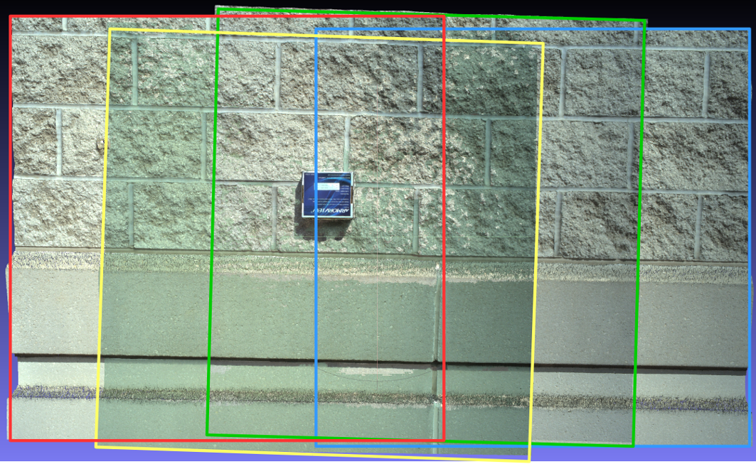
Figure 1 Aligned point clouds. Colored rectangles are the indicator of the individual point clouds. ↑
In figure 1, each point cloud is enclosed into a colored rectangle. The point cloud marked by the yellow rectangle shows a sort of green color because the sun came out of the cloud in the sky and the camera was performing auto exposure adjustment at that moment.