Some useful CGAL functionalities for working with point clouds and surface meshes
Introduction
Recent work requires lots of processing on point clouds, including sampling, filtering, and surface reconstruction. Most of the codes are composed by using PCL at the beginning. Later, more and more processing involves mesh manipulation. Then I came across CGAL. Never used but I knew its existence. CGAL turns out to be extremely powerful and versatile, however at the same time, hard to understand due to its heavy use of C++ template meta-programming. It causes some headache, and possibly reduces my hair coverage, while I am trying to learn and use CGAL. This blog shows some of my own experiences with CGAL, particularly on aspects related to point cloud processing.
The content includes:
- Read and write point cloud with PLY format with point properties
- Read and write surface mesh.
- Surface mesh property map and normal estimation.
- Mesh check and repair.
- Advancing front surface reconstruction.
- Isotropic remeshing.
- Surface mesh hole identification and filling.
- Ray shooting to a surface mesh.
- Shape detection from a point cloud.
CGAL’s official site provides detailed documentations including tutorials and user references on every package. I will borrow a lot of content from the official documentation, implementing the code, and adding my own comments on the usage.
I want to acknowledge that the CGAL mailing list is extremely helpful. The experts there are responsive and active, once you’ve found yourself in a corner of code and could not make out any sense of it, then the ultimate resort is the CGAL mailing list.
The cover image of this post is copied from the CGAL offical site.
Sample code
I prepared a Github repo that holds all the sample codes discussed in this blog. I am working on Ubuntu 18.04 and CGAL 5.1. To compile the code, a system environment variable should be defined as CGAL_DIR showing where CGAL is located in the filesystem.
Source of sample data
Some of the point clouds and meshes in this blog are copied from the sample files of Meshlab. All rights reserved to the original authors.
The sample data should be placed in the Data sub-directory of the source code. All the data and results from running the sample codes could be downloaded from here.
Read and write point cloud with PLY format with point properties
The first task is how to get points in and out of CGAL. For me, I usually use the PLY format as my primary point cloud file format since it has the ability to store various per-point properties and we also can save mesh into PLY files. So doing IO with PLY files is the first thing I’d like to discuss.
Here I provide a sample code showing the process.
It seems to me that, unlike PCL, CGAL leaves the job of defining the type for 3D point representation to the user and try to be flexible and at the same time. A point cloud in CGAL is nothing but a collection of points, however, we have to define the type for “point”. CGAL kernel already provides users the basic point representation being Kernel_t::Point_3 is the sample code. So we could represent a point cloud as a std::vector<Kernel_t::Point_3>. Normally, a point cloud also has additional properties other than the coordinates of points, e.g. point normal and color. For those additional properties, CGAL expects us to just define a std::tuple and put any property we want in the tuple, then make a container of this tuple type as the point cloud.
As for normal vectors, we could use Kernel_t::Vecotr_3. For color, however, depending on how many color channels you want, you could use std::array< unsigned char, N > where N could be 3 or 4 (an additional alpha channel).
For 3D points and normals, CGAL provides helper functions CGAL::make_ply_point_reader() and CGAL::make_ply_normal_reader() for reading and similar helpers for writing. For a std::array represented color, however, we have to be more specific on how CGAL is supposed to read and write data. Specifically, during the call to CGAL::read_ply_points_with_properties(), we will use helper function CGAL::Construct_array(). For writing the color property, we have to implement CGAL::Output_rep class so that CGAL knows how to deal with the color type. Please refer to the sample code for more details.
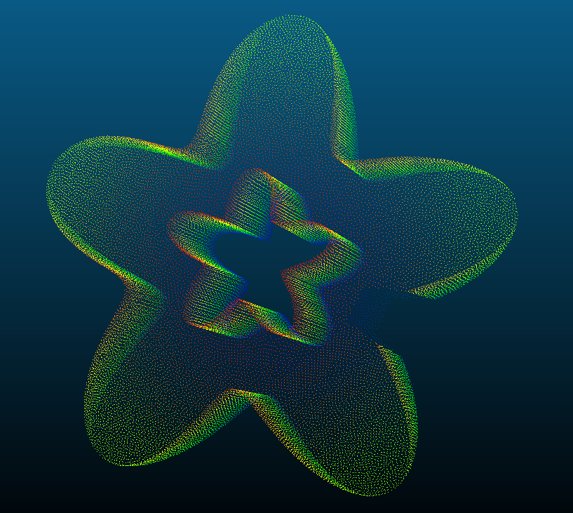
The sample code reads a point cloud in PLY format and writes it back to the filesystem as it is. So we could load the files into point cloud visualization software such as CloudCompare to check if we are reading and writing the point clouds properly. I noticed that the size of the output PLY file is larger than the input. This might have something to do with the underlying CGAL kernel we are using and the kernel is using a double-precision floating-point type. The following is a sample point cloud, Data/PointClouds/TrimStarInit0.5_NormalColor.ply.
To test with the sample point cloud shown above, we could use the following commands.
<path to executable>/ReadWritePLYPointCloud \
	<path to repo>/Data/PointClouds/TrimStarInit0.5_NormalColor.ply \
	<output filename>
Read and write surface meshes in PLY format
Read and write surface meshes in PLY format is made really simple in CGAL, the Surface Mesh package provides the dedicated APIs for these purposes, namely, the CGAL::read_ply() and CGAL::write_ply() functions.
The sample code for using these two functions is here.
If we put a sample mesh, T_d.ply, in Data/Meshes, then we can invoke the sample program by
<path to executable>/ReadWritePLYMesh \
<path to repo>/Data/Meshes/T_d.ply \
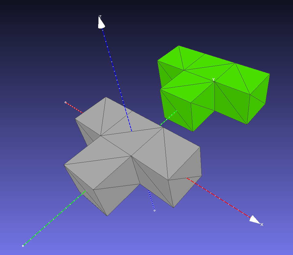
<output filename>This mesh is one of the sample meshes of Meshlab. It is basically a set of blocks in a T-shape layout. To illustrate some interesting usage of CGAL, I modified the original mesh by adding a new vertex property called “d” with float property type. During the reading process, CGAL handles this new vertex property automatically for us and a property map with the name v:d will be created. In the sample code, we try to get access to property map v:d and print out all the values. The values start from 100 and end at 119 (20 vertices in total).
CGAL handle entities such as points, vertex normals, face normals as property maps. The actual 3D points are saved as a vertex property map called v:point. CGAL has conventional names for frequently used properties such as v:normal and f:normal with f: being a face property map. So as been said, if we want to access the point of a vertex, it is normally done through the v:point property map. From my experience, CGAL provides no method to directly modify the coordinates of a point (the Kernel_t::Point_3 in the sample code). If you really want to do that, make a new Kernel_t::Point_3 and overwrite the original object in the v:point property map. I add 6 to all the y-coordinates of the original mesh vertices.
The sample code writes the modified mesh to the filesystem in both ASCII and binary format. If we load the mesh into Meshlab, we will see something like the following, with the green mesh being the modified mesh (the color is assigned in Meshlab). To write a binary PLY file, it seems that we also have to use the CGAL::set_binary_mode() method. Please refer to the sample code for details.
One additional thing we could observe from the result ASCII PLY file is that CGAL does use double-precision floating-point numbers.
Surface mesh property map and normal estimation
In the previous example, we see that CGAL manages the point associated with mesh vertices as a property map. The same treatment is used for mesh surface normals.
Once we have a mesh, a normal estimation is straightforward. The tricky part is how to determine the direction of individual normals if the underlying mesh is not a closed surface. That means we have holes in the surface mesh and we are not allowed to fill the holes or filling is impossible. I do not have good solutions for this issue at the moment.
Anyway, we could ask CGAL to help us to estimate the surface normals of a surface mesh. You can do face normals and vertex normals. The sample code is here. To run the executable, follow the commands
<path to executable>/SurfaceNormal \
	<path to repo>/Data/Meshes/bunny10k.ply \
The input mesh is one of the sample meshes of Meshlab. This particular mesh has over 1000 isolated vertices. For face normal estimation, all facets will be associated with normal vectors stored in a property map. However, for vertex normals, no normal vectors are generated for the isolated vertices. This is shown in the output information that the executable prints (the [0, 0, 0] normal vectors).
Hello, SurfaceNormal!
main: Estimate face normals.
estimate_face_normal: Create surface normals.
*iterFN = -0.221231 0.974061 -0.0475518
*iterFN = -0.367694 0.916929 0.155058
*iterFN = -0.21876 0.970464 -0.101705
*iterFN = -0.349913 0.930575 0.107661
*iterFN = -0.250127 0.903394 0.348304
*iterFN = -0.148972 0.915857 0.372845
*iterFN = -0.237273 0.745088 0.623334
*iterFN = 0.361002 0.925663 0.113253
*iterFN = 0.749282 0.634487 0.189744
*iterFN = -0.678005 -0.210922 -0.704146

main: Estimate vertex normals.
estimate_vertex_normal: Create vertex normals.
Sequentially list the sample vertex normals:
*iterVN = 0 0 0
*iterVN = 0.429513 0.20134 0.88033
*iterVN = 0 0 0
*iterVN = 0 0 0
*iterVN = -0.734201 -0.0354185 -0.678008
*iterVN = 0 0 0
*iterVN = 0 0 0
*iterVN = 0 0 0
*iterVN = 0 0 0
*iterVN = 0.657728 0.0222236 0.752927
List the sample vertex normals according to the vertex descriptors.
vertexNormalMap[v] = 0 0 0
vertexNormalMap[v] = 0.429513 0.20134 0.88033
vertexNormalMap[v] = 0 0 0
vertexNormalMap[v] = 0 0 0
vertexNormalMap[v] = -0.734201 -0.0354185 -0.678008
vertexNormalMap[v] = 0 0 0
vertexNormalMap[v] = 0 0 0
vertexNormalMap[v] = 0 0 0
vertexNormalMap[v] = 0 0 0
vertexNormalMap[v] = 0.657728 0.0222236 0.752927

The mesh is invalid.
nIsolatedVertices = 1113

main: Estimate the vertex normal again.
estimate_vertex_normal: Retrieve vertex normals.
Sequentially list the sample vertex normals:
*iterVN = 0 0 0
*iterVN = 0.429513 0.20134 0.88033
*iterVN = 0 0 0
*iterVN = 0 0 0
*iterVN = -0.734201 -0.0354185 -0.678008
*iterVN = 0 0 0
*iterVN = 0 0 0
*iterVN = 0 0 0
*iterVN = 0 0 0
*iterVN = 0.657728 0.0222236 0.752927
List the sample vertex normals according to the vertex descriptors.
vertexNormalMap[v] = 0.429513 0.20134 0.88033
vertexNormalMap[v] = -0.734201 -0.0354185 -0.678008
vertexNormalMap[v] = 0.657728 0.0222236 0.752927
vertexNormalMap[v] = 0.984743 0.112655 0.132625
vertexNormalMap[v] = 0.246174 0.330777 0.911035
vertexNormalMap[v] = 0.914411 0.25762 -0.312224
vertexNormalMap[v] = 0.00329743 0.469879 0.882725
vertexNormalMap[v] = 0.269242 0.241589 0.932279
vertexNormalMap[v] = -0.14863 0.611228 0.777374
vertexNormalMap[v] = -0.360826 0.582433 0.728407
After we remove the isolated vertices from the original surface mesh but do not change the storage structure of the vertex normal property map, the property map still holds the data for the removed vertices. But at this moment, the mesh will not have the vertex descriptors that get mapped into the isolated vertices before the removal. Thus, the way I designed the sample code wastes the storage for the isolated vertices.
One piece of advice, when estimating the vertex normals of a surface mesh, it might help if we first remove all the isolated vertices. I did not test degenerated meshes yet. Maybe in the future.
Mesh check and repair
In the last sample, we’ve seen how to remove isolated vertices from a surface mesh. Apart from isolated/dangling vertices, I also found some other defects that are easy to be encountered in my workflow. They are non-manifold vertex and self-intersection. To deal with these defects, CGAL has provided us dedicated tools. The way for handling a non-manifold vertex is to make a copy of the vertex and distribute the original edges to the newly create vertex to make the vertex manifold. For self-intersections, the treatment is usually a detection and removal. CGAL also provides a function CGAL::is_valid_polygon_mesh() to check the validity of a surface (polygon) mesh, respect to the connectivity and integrity of the mesh. When we have isolated/dangling points, CGAL::is_valid_polygon_mesh() returns false (as shown the surface normal sample). But is seems to return true with self-intersections and non-manifold vertices.
Here I prepared a piece of mesh which is obtained from a Screened Poisson Reconstruction. The mesh has lots of self-intersections and a bunch of non-manifold vertices. Let’s go and repair them. The sample code is here. To run the executable, use
<path to executable>/Repair \
	<path to repo>/Data/Meshes/PillarSurface.ply \
	<path to repo>/Data/Repair/Repaired.ply
The terminal should show
Hello, Repair!
Collecting intersected faces.
547 faces to be removed.
Begin removing intersected faces.
Removal done.
Begin duplicating non-manifold vertices.
newVerticesNB = 27
Advancing front surface reconstruction
To get a surface mesh from a point cloud, we have to do a surface reconstruction. CGAL provides multiple choices for reconstruction. In my processing pipeline, the point cloud is first downsampled, resulting in a nearly uniformly distributed point cloud. And also, I want the reconstructed surface to cover the point cloud region only, not extending the surfaces into the void space, However, it is OK to fill some small gaps or holes in the process. So the advancing front surface reconstruction (AFSR) is the way to go.
To use AFSR, one needs to provide two helpers. One of them works as a checker for distance and it seems to help us to achieve the Delaunay criteria. In the sample code, it is called PriorityRadius. The other helper serves as a constructor that takes 3 vertices and construct a single facet at one time. This constructor is called MeshConstructorByPointIndices.
To test the sample code, I cut a small portion off the Star sample provided by Meshlab. The point cloud is the same one used for testing the point cloud IO. The point cloud has surface normal and color encoded, but I only need the points. So it is a little bit different from the implementation in the previous point cloud IO sample. After reading the point cloud, the AFSR is triggered. Finally, the reconstructed mesh is saved to the filesystem as usual.
Note that this sample has a significant execution time difference between the debug and release builds. On my current computer, the debug build costs about 1min while the release build needs less than 1s. To run the executable, use the following commands.
<path to executable>/AFSReconstruction \
<path to repo>/Data/PointClouds/TrimStarInit0.5_NormalColor.ply \
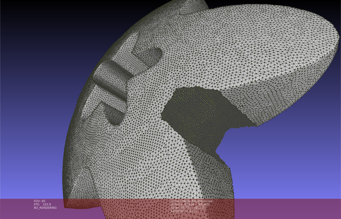
<path to repo>/Data/AFS/Reconstructed.plyThe following figure illustrates the reconstructed surface and the input point cloud (dark green colored points, maybe hard to see the color) in Meshlab.
Isotropic remeshing
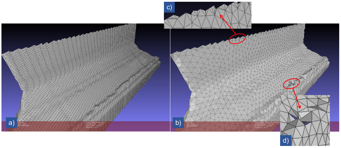
Of course, CGAL has the function for isotropic remeshing. However, we have to be careful that it only works when the mesh passes the test of CGAL::is_valid_polygon(). The official tutorial shows shat we could try to split the long border edges before remeshing the interior. The split borders are then fixed during the isotropic remeshing. The sample code is basically re-implementing the official tutorial. We could take the output mesh of the mesh repair sample as the input for isotropic remeshing. Note that after the isotropic remeshing, there might be defects including self-intersections and non-manifold vertices. We could do the repair in the way we did for the repairing sample. The following figure shows the meshes before and after the isotropic remeshing. I marked out the borders and the defect regions on the remeshed surface.
Surface mesh hole identification and filling
Surface meshes are represented as halfedge graphs in which holes are actually equivalent to mesh bounaries. For a halfedge graph in CGAL, all bounary halfedges are connecting a regular facet and a special null facet. All the bounariy halfedges taking the same null facet as the incident facet. To identify a hole, starting from a boundary halfedge, and follow the “next halfedge” until reaching the starting halfedge (a circle is formed). CGAL::Halfedge_around_face_circulator<> provides the circulator for traversing the halfedges. This strategy is actually used inside the hole-filling APIs of CGAL.
// Let Mesh_t be the typedef of the mesh type and variable mesh be the mesh object.

typedef boost::graph_traits<Mesh_t>::halfedge_descriptor HalfedgeDesc_t;
typedef CGAL::Halfedge_around_face_circulator<Mesh_t> HalfedgeAroundFaceCirculator_t;

for ( HalfedgeDesc_t h : halfedges( mesh ) ) {
	if ( !is_border(h, mesh) ) {
		continue;
	}

	HalfedgeAroundFaceCirculator_t circ ( h, mesh ), done(circ);

	do {
		// Do stuff.
	} while ( ++circ != done )
}
I was using one of the CGAL’s hole filling APIs, CGAL::Polygon_mesh_processing::triangulate_and_refine_hole(). As the name suggests, it triangulates the identified hole and refines the newly created mesh. In my workflow, after the holes are filled, I’d like to do an isotropic remeshing only for the newly created facets in the hole areas. Then retrieve the vertices of the remeshed facets, save the points of the vertices into a separate file. All these actions could be realized by the previously discussed contents of this article.
As always, there is a sample code showing the hole filling, selected remeshing, and point collection. To run the sample code, the user needs to specify the input mesh and the output directory. Let’s take the resulting mesh from the AFS reconstruction as the input mesh, the commands will look like
<path to executable>/HoleFilling \
<path to repo>/Data/Meshes/AFSReconstructed.ply \
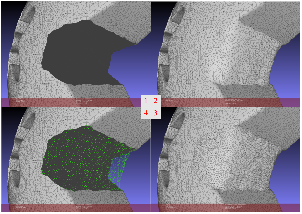
<path to repo>/Data/HoleFillingThere is only one large hole on the surface mesh. The following figure shows the original mesh with a hole, initially filled hole, remeshed hole area, and the retrieved points, respectively.
Ray shooting to a surface mesh
Some tasks require projecting pixels from an image into the 3D scene. These pixels could be the result of some kinds of 2D detection or segmentation tasks. With the camera pose, camera intrinsic parameters, and, of course, the 3D surface mesh, we cloud project those pixels onto the surface mesh with the ray shooting APIs, of the so-called “3D Fast Intersection and Distance Computation (AABB Tree)” APIs, of CGAL.
During the preparation of this sample, I tried to make some images from Meshlab and let Meshlab create the intrinsic and extrinsic (pose) parameters for the cameras. I had some trouble to make the whole pipeline work, there were always some weird things happening when I transformed the camera. Anyway, I managed to generate a dummy camera, its 3D pose (and orientation), and the pixels that need to be projected. The target mesh is the bunny10k mesh provide by Meshlab. Every pixel and the origin point of the camera (the camera center) make a 3D direction vector. The projection is done by shooting a ray starting from the camera origin along the direction vector. If the ray hits the surface mesh, the first intersection point is retrieved as the projected point.
In the sample code, I additionally calculated the surface normal of the mesh. Then after a pixel is projected to the surface mesh, the projected point is shifted along the local surface normal direction by a small amount of distance. In this way, the projected point is made floating above the surface mesh and becomes easily visible. There are relatively more input arguments than the other samples
<path to executable>/RayShooting \
<path to repo>/Data/Meshes/bunny10k.ply \
<path to repo>/Data/Meshes/Meshlab/CameraPoseT.dat \
<path to repo>/Data/Meshes/Meshlab/CameraIntrinsics.dat \
<path to repo>/Data/Meshes/Meshlab/CirclePoints.csv \
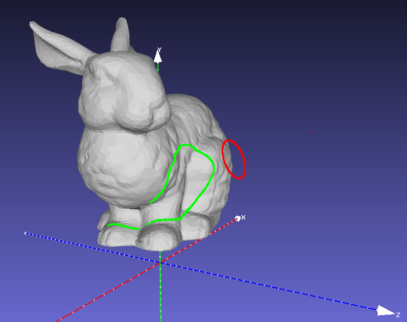
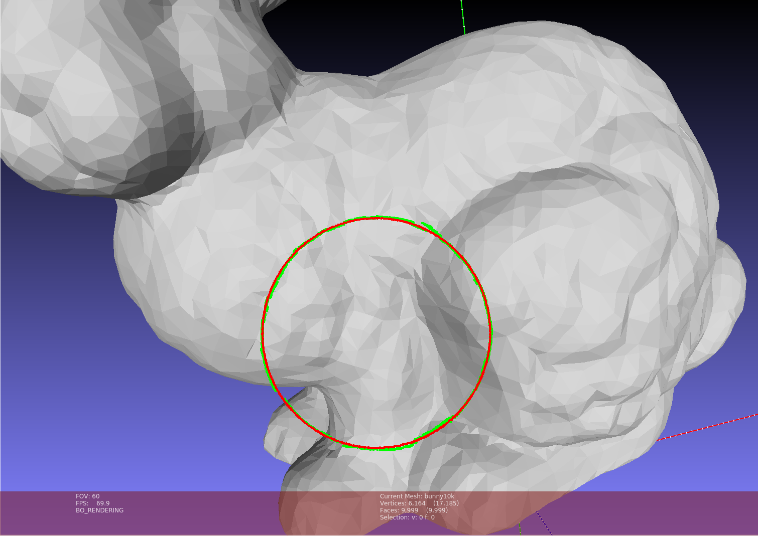
<path to repo>/Data/RayShooting/HitPoints.plyAfter execution, two point clouds will be written to the file system. One for the camera origin and the direction points (direction vectors are scaled). The other point cloud is the project points. The following two figures show the camera origin point (red), direction points (red), and the projected points (green) from a side view and front view. This particular sample has 3615 hits and 87 misses.
Shape detection from a point cloud
CGAL actually provides several kinds of primitive shape (e.g., planes and cylinders) detection methods for different underlying geometries. Some methods work on point clouds and surface meshes. However, the methods for surface meshes work in a way that they try to collect facets into clusters falling in the same primitive geometry such as planes. What I really wanted for my project is detecting shapes from the vertices of a surface mesh. Well, that just means we need to extract points from the surface mesh vertices and then do our shape detection from the points. CGAL names the module as “Efficient RANSAC”. When operating on a point cloud, it needs the point normal to work properly. In this sample, I’m gonna estimate the normals on the surface vertices before point extraction. We do not orient the normal vectors since shape detection should not sensitive to the direction (inwards or outwards) of the vectors. Then points are extracted from the vertices and the vertex normal property is copied to the point cloud. I only do plane detection. After the detection, every point is assigned a color representing its plane association (plane index). Finally, the point cloud with normal vectors and color is written to the file system for visualization.
To run the sample code, all you need is
<path to executable>/PCShapeDetection \
	<path to repo>/Data/Meshes/Bar.ply \
	<path to repo>/Data/ShapeDetection/ColoredPoints.ply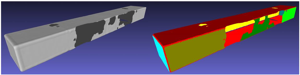
Closing remark
Well, I think that’s it. CGAL, with its glowing charm, does give me some trouble when I started to work with it. However, as time goes, it becomes better. Still, CGAL is unlike the other packages that I am using, it has its own characteristics and there exists lots of stuff that I do not fully understand. Yet, the portions of CGAL I managed to use may be forgotten after a while. That’s partially the motivation when I start to write this post over three weeks ago, to make a note for myself and think it through again. I want to express my gratitude, again, that the CGAL mailing list is very active and helpful. Thank you there!
Keep safe, keep active!