Simple optical flow based on depth and pose information
Recently, I was helping to implement a simple program that performs optical flow calculation between frames of video images with the help of known depth and pose information associated with the images.
Let us define the first frame as Frame 0, and the second to be Frame 1. And for my current task, the camera is under constant movement. For optical flow, it is usually represented by a color image with HSV color space. In this image, Channel H (Hue) is used to represent the flow direction of the individual pixel of the Frame 0. That is if the camera is moving, every pixel of Frame 0 seems to move with respect to Frame 1 and exhibiting a representative color regarding the flow direction. Channel V (Value or Lightness) tells the magnitude of the movement of a pixel. The larger the movement, the brighter it should be. We leave the S (Saturation) Channel to be its highest value and never touch it.
The thing is, once you know the camera pose and depth information of each frame, you know everything. No fancy algorithm is needed to perform optical flow calculation since you can calculate the movement of the individual pixel. The overall process looks very much like the following.
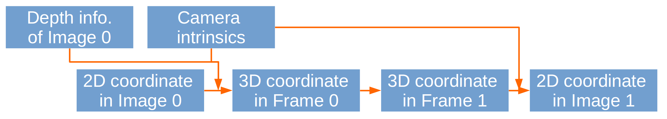
Figure 1 The flow chart. ↑
As shown in figure 1, the overall process is really straightforward. If the camera is rectified and has no distortion, all of the transformations could be expressed by simple linear algebra expressions.
Actually, the images are extracted from video frames recorded in the Unreal Engine. We are simulating a UAV in Unreal with the help of AirSim, an open-source project implementing drone simulators. AirSim is maintained by Microsoft. The video stream comes from the virtual camera mounted on the simulated UAV in Unreal. Individual frame images are extracted from the video stream, with associated depth and camera pose information. Two sample image frames are shown in figure 2.
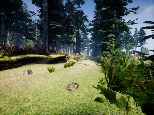
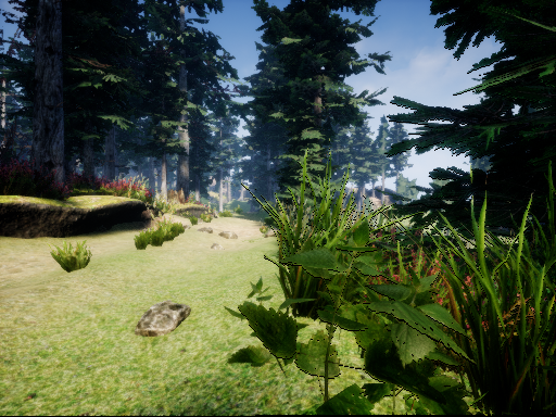
Figure 2 Original frame images. Top: first frame, bottom: second frame. ↑
As one can easily perceive, the camera has a yaw movement from left to right direction. The global coordinate system is defined in such a way that the z-axis is pointing downwards. Then this yaw movement is represented by a rotation with positive angle value along the z-axis. The resulting optical flow image may look like figure 3. The values for the H and V channels of the resulting HSV image are calculated in a way similar to one of the OpenCV tutorials.
Figure 3 The optical flow. ↑
The color in figure 3 shows that all the pixels of Image 0 are moving in roughly the same direction. In this case, the direction is from left to right. The brightness of figure 3 shows the magnitude of pixel movements. For pure yaw movement, the close a pixel locates to the vertical center line of the image, the less it moves in magnitude.
Since we have these data, we could do something else like computing the 3D point clouds based on Image 0 and 1. We could import these point clouds into MeshLab and check the consistency between the depth and cameras poses. The point clouds may look like figure 4 and figure 5.
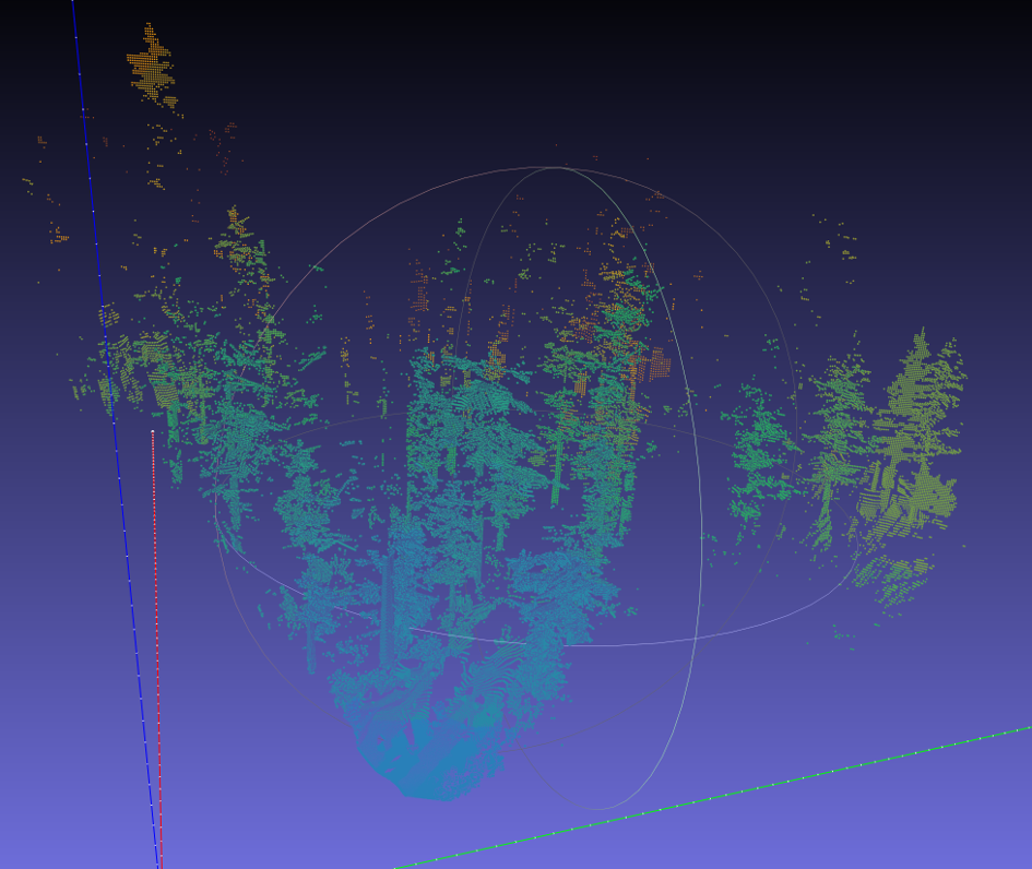
Figure 4 Point cloud of Image 0. ↑
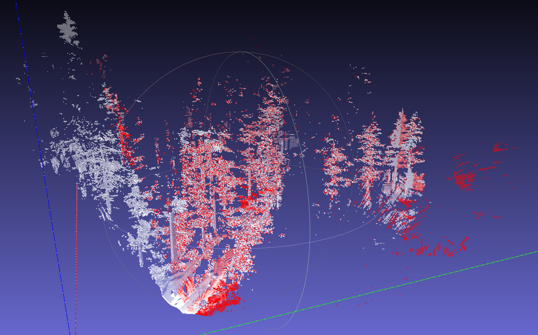
Figure 5 Point clouds of Image 0 and 1. White: Image 0. Red: Image 1. ↑
In figure 4, I use color to indicate the distance from the camera. Blue means points are near the camera and red means far away. I generate my own color mapping method with the help of this post. In figure 5, the two point clouds get aligned, meaning that the depths and camera poses are consistent with each other. Good job.
One other thing one may do with these data is warping Image 0 to Image 1. After obtaining the optical flow between the two images, we could easily warp Image 0 and see how it will look like from the perspective of Image 1. Figure 6 shows the result of warping.
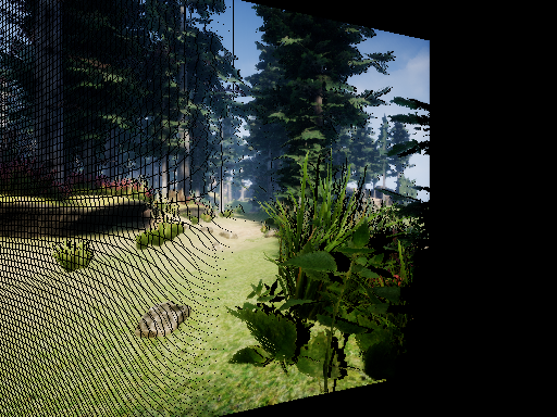
Figure 6 Warped image. ↑
In figure 6, all the regions that could be seen originally in Image 0 but could not be perceived in Image 1 are rendered black. The pixels of Image 0 move to their new locations in Image 1. Since the camera is rotating from left to right, objects in the camera view will move to the left. The black ripples in figure 6 are the result of transformation with discretized pixels, pixels originally located at the left of Image 0 simply could not cover a relatively larger area in Image 1, leaving holes after warping.
This work is done with the help of Wenshan Wang.