Fully connected artificial neural network

Artificial intelligence or data-driven modeling is so hot these days. I find it is so magical that I decided to learn some basics and give it a try.

In this post, I will discuss the implementation of a fully connected artificial neural network (FCANN). For the activation functions, the ReLU functions is used. For the loss functions, the sum-of-squares and the cross entropy with Softmax are used. The neural network (NN) is trained by on-line backscatter propagation (BP) method. To demonstrate the FCANN, first I tried to train a NN by data obtained from the sine function. Then, another NN was trained to recognize hand-written numbers from available labeled data set.

Fully connected artificial neural network

The concept of FCANN is so straight forward that there is no need for in-depth explanation. Some specific concepts must be defined to fit this particular post. The input is a vector X, the output of the NN is a vector y and the training data is expressed by Y. For classification, y and Y are transformed by the Softmax function.

For the BP method, the most important thing is obtaining the partial derivatives of the loss function with respect to the model parameters (\(w_{mn}^j\) and \(b_{n}^j\)). This could be discussed by the following short article.

• Download the PDF file.

For on-line backscatter propagation, the corrections of weight w is expressed by

\[ w_{mn}^{j} := w_{mn}^{j} - \alpha \cdot \frac{\partial L}{\partial w_{mn}^{j}} \]

where \( w_{mn}^{j} \) is the weight parameter in the \( j^{\mathrm{th}} \) layer. \( \alpha \) is the learning rate. \( \alpha \) should be a positive real number, typically ranging from 0 to 1. This correction is performed for each training data, following the on-line backscatter propagation scheme. For \( b_{n}^j \), the correction method is similar.

\[ b_{n}^{j} := b_{n}^{j} - \alpha \cdot \frac{\partial L}{\partial b_{n}^{j}} \]

In the training stage, the training data is fed into the NN (feed forward), then the loss of the output of the NN is evaluated. Next is the calculation of the gradients of \(L\) with respect to the model parameters. Then we perform backscatter propagation. The loss is constantly monitored and a convergence of training is reached when the loss value drops below a certain level.

At this moment, I do not use some fancy open-source packages to do the trick. Only plain python with NumPy is used. The source code could be found here (GitHub Repo). The code may be under continuously modification since I am planning to add new features.

Learning of a sine curve

As a beginning, let’s start with learning a sine curve. The training data is very straight forward, it is the sine values with the dependent variable ranging from 0 to \( 2 \pi \). 1000 evenly spaced points are set as the input to calculate the corresponding sine values. These 1000 pairs of data points are used as the training set. We can use this set of training data multiple times to train an NN. Furthermore, we could randomize the order of the data set every time we feeding the data into the NN.

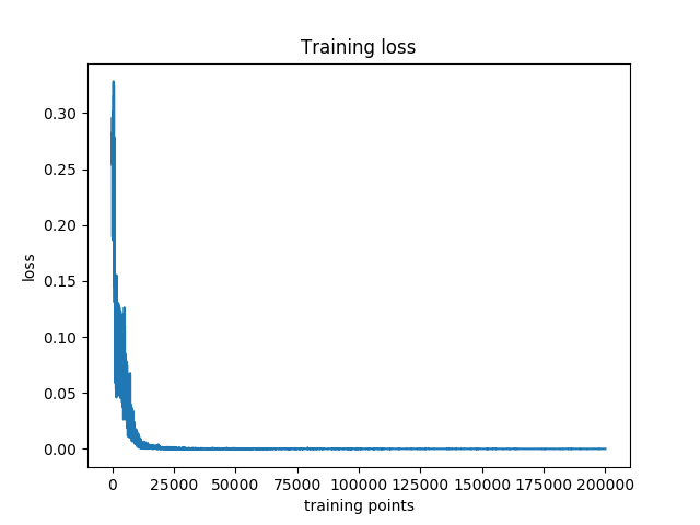
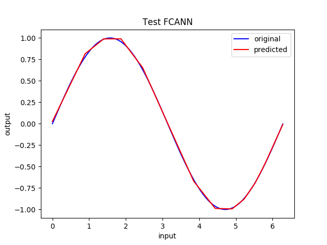
A FCANN with 2 hidden layers and 10 neurons in each layer is set up. For the hidden layer the ReLU activation function is utilized and no activation function for the output. The sum-of-squares loss function is used. After training the NN 200 times, each time I applied the above training set in its randomized order, we could get a working NN. The following figures show the loss history and the testing results of the trained NN. 2000 evenly spaced points within 0 and \(2\pi\) are used as input to test the trained NN. Good agreement is found between the original and predicted curves.

Learning of hand-written numbers

The training set is a bunch of labeled grayscale images which are similar to the following figure.

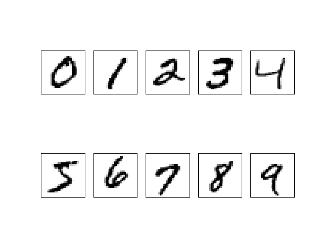
Each image in the training set is a 28x28 pixels graph. And the image is represented by a 2D NumPy ndarray with its values ranging from 0 to 255. The input of the NN is simply the reshape of the ndarray, and it falls into a column vector. Since this task is essentially a classification, the output of the NN is designed to be a column vector with 10 components. Each component of the output vector stands for a possibility of a specific number, 1 for the highest possibility and 0 for not possible. For example, the following column vector stands for Number 0 (superscript T means transpose).

\[ [ 1, 0, 0, 0, 0, 0, 0, 0, 0, 0 ]^{\mathrm{T}} \]

And the following vector is equivalent to 7.

\[ [ 0, 0, 0, 0, 0, 0, 0, 1, 0, 0 ]^{\mathrm{T}} \]

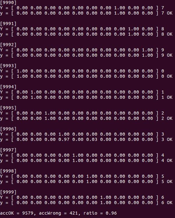
The cross entropy loss function with Softmax is quite suitable for this kind of task. The expressions relating to cross entropy is listed in the above PDF file. The important thing is that while evaluating the loss of the prediction of the NN, the output of the NN is firstly transformed into a vector similar to the above two vectors, by applying the Softmax function. Then the loss value could be calculated. The output of the trained NN also has to be transformed by the Softmax function to perform the classification properly. The output of the trained NN, after applying the Softmax function, should has one component with predominant value (close to 1) and all other components with relatively small values (near to 0).

This time a FCANN with 2 hidden layers has been built and trained. There are 100 neurons in each layer. The activation function is ReLU and, again, the activation function for the output is omitted.

There are 60000 images in the training set and another 10000 for testing. The FCANN is trained for two times on all the 60000 inputs. Then a benchmark run of prediction on the testing set shows that the rate of successful prediction is about 96%.

At the last

This post is my first attempt to implement an ANN. It is so delightful when I see the prediction of my NN is correct on the testing data set. Yeah, it feels good and I want more.

NEXT: The Convolution Neural Network.

Special thanks: My mentor of artificial intelligence and machine learning, Wenshan Wang.