Rotordynamic analysis using ANSYS Workbench with solid finite element

Rotordynamic analysis using ANSYS Workbench with solid finite element

We have discussed the rotordynamic modeling process in my previous post. In that post we adopted ANSYS Mechanical APDL environment and built our model with 2D beam element. In this post I would like to talk about the modeling method using solid finite element in ANSYS Workbench environment.

The major difference between modeling with APDL and Workbench includes

(1) The way we handle the bearing and running clearance.

(2) Displacement boundary condition.

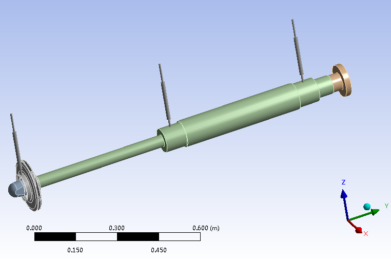
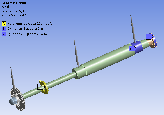
Let’s use the same sample rotor in the previous post. Drag and drop a ‘Modal’ box onto the project schematic area, import the geometry. The imported modal should be looked like those in the following figure.

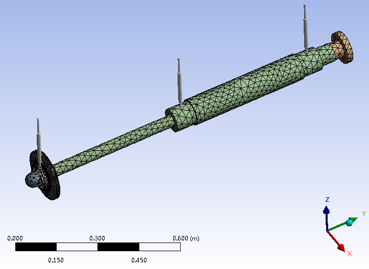
The above figure also shows three newly added longitudinal Body-Ground springs. These spring elements represent the two roller bearings and the running clearance of impeller ring. These spring elements are inserted in the ‘connections’ group of the left tree view of the simulation project. By default, these spring elements are later implemented by Combin14 elements. We have to change them into Combi214 elements. Further, the supporting effect of the running clearance depends on the rotating speed of the rotor. Thus, we have to create a data table to represent the speed dependent property. The above desired modifications are done by inserting a ‘Commands’ node under the last spring element node in the left tree view.

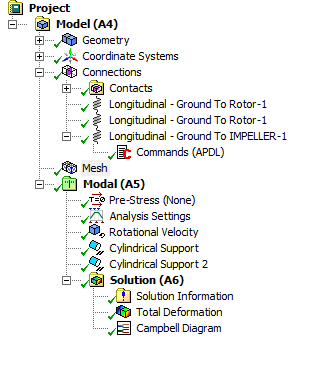
In the ‘Commands’ node, we use APDL commands to find every Combin14 element, change its type into Combi214, then alter its settings according to the type of supporting which could be either bearing of running clearance. The order that the original spring nodes appear on the list under ‘connections->Contacts’ group determines the creation order of these spring elements. And this is the only way we can distinguish each spring element.

Content of a sample ‘Commands’ node are provided here

For displacement boundary condition, we could use the ‘Cylindrical Support’ functionality that provided by ANSYS Workbench. I apply this kind of displacement boundary condition on the round surface of the coupling. For this ‘Cylindrical Support’, the radial and axial constraints are eliminated leaving only the tangential constraint. And another ‘Cylindrical Support’ is applied on the round surface of the upper bearing. This time only the axial constraint is kept.

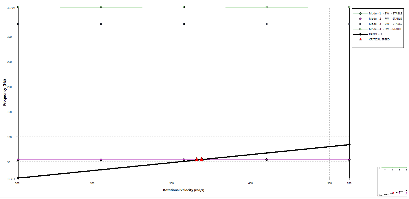
The calculate Campbell diagram is listed below.

After configure the ‘Modal->Analysis Settings’ node to turn on functionalities such as number of modes wanted, damping and Coriolis effect. For critical speed analysis, the rotating speed range is set afterwards.

We can then calculate the modal solution and let ANSYS workbench plot a Campbell diagram.