Rotordynamic analysis using ANSYS Mechanical APDL with the rotor modeled by beam element

Rotordynamic analysis using ANSYS Mechanical APDL with the rotor modeled by beam element

The rotordynamics of rotating machinery is one of the key issues that guarantee safe operation. One would like to know the rotordynamic characteristics of a new unit in its design phase. Generally for a pump unit, two aspects of rotordynamics are of particular interests: damped critical speed and damped unbalance response. These two terms are defined in classic text books of rotordynamics and could be obtained by conducting lateral vibration analysis.

Here I would like to perform an illustrative analysis of a imaginary pump rotor using the software ANSYS Mechanical APDL. For the rotor, one can actually choose either beam or solid element. I will utilize beam element in this post. As for solid element, I prepared another post in which the ANSYS Workbench is adopted.

Official help and documentation

One could find relative content in ANSYS’s official help and documentation. The documentation has a special chapter discussing detailed instructions and examples needed to perform rotordynamic analysis with ANSYS Mechanical APDL.

In this post, I would like to emphasis on some topics that are hard to find references or easy to make mistakes.

List of content

• Imaginary pump rotor
• Overview of major steps
• Rotor
• Rotating component
• Bearing
• Damped critical speed analysis
• Damped unbalanced response

Imaginary pump rotor

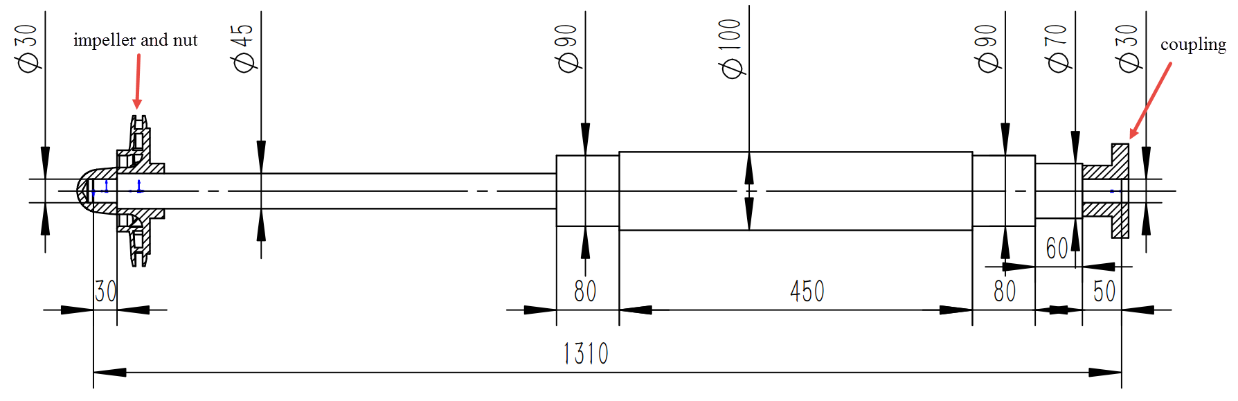
We could take an overhang configuration as the imaginary pump rotor. Overhang means that the impeller of the pump is installed outside the range of supporting bearings and it could be illustrated in the following figure. The two rotating components are the impeller and coupling. The rotor is supported on two roller bearings. The major dimensions are also listed in the figure.

Overview of major steps

The major steps of the modeling process are as follows:

• Rotor.
• Rotating components.
• Bearings and other supporting components.
• Calculation settings.
• Post-processing.

Rotor

The rotor or shaft could be modeled using BEAM188 element provide by ANSYS Mechanical APDL. In order to properly generate a rotor model the rotor material parameters should be set with MP command. The user has to choose different beam cross-section type according to the actual rotor by issuing SECTYPE and SECDATA commands. The value of argument “type” of SECTYPE command is BAEM. And the value of argument “subtype” of SECTYPE should be “CSOLID” when the corresponding rotor section is solid and “CTUBE” when the rotor section is hollow. After specify each beam node by N command the BEAM188 element could be created by E command.

Rotating component

The main rotating components consist of two parts, the pump impeller on one end and the coupling on the other.

In ANSYS Mechanical APDL, rotating components could be modeled by the single node MASS21 element. I, personally, think that it is practical to set KEYOPT(3) of MASS21 element to be 0 and input MASSX, MASSY, MASSZ, IXX, IYY and IZZ by hand. Here MASSX, MASSY and MASSZ should be identical. As usual, MASSX to IZZ are specified by R command. Finally, MASS21 element is created by E command after choose the right element type by ET command.

Bearing

ANSYS Mechanical APDL has provided the user with the COMBI214 element to model the stiffness and damping effects of bearing in rotating structure.

COMBI214 element needs only two nodes, one on the rotor and the other on non-rotating structure. Usually we do not model the non-rotating structure for a rotordynamic analysis and we have to create imaginary dummy points (by N command) in order to use COMBI214 element. It is actually pretty tricky when create COMBI214 element that the user has to explicitly specify the two nodes in the right order. According to the specification of COMBI214 element, when creating COMBI214 element by E command, the first node is non-rotating.

Another notable aspect of COMBI214 element is that the user has to specify the working plane. It is accomplished by setting KEYOPT(2). The user should make sure that the two points of a COMBI214 element lie in the plane specified by the associated KEYOPT(2). It is important to check the actual coordinate of each node since ANSYS Mechanical APDL has very tight tolerance when testing the positions of COMBI214 nodes. This situation gets erroneous when we use ANSYS Workbench to perform rotordynamic simulation.

It is the user’s choice that where the non-rotating node of COMBI214 element should be. However, it seems that ANSYS Mechanical APDL expects the two nodes to be at exactly the same place in 3 Dimensional space. Otherwise, it complains with warning in the log file.

The real challenge comes up when we are setting the stiffness and damping parameters of COMBI214 element. There are three key aspects I want to talk about.

• Set KEYOPT(3)

  It is good practice to set KEYOPT(3) to be 1. This tells ANSYS Mechanical APDL that the stiffness and damping parameters are not symmetric. Then we input every stiffness and damping parameter using real constant.

• Set real constant with both R and RMORE commands

  The real constants of COMBI214 element have 8 individual values. It is notable that the leading 6 parameters are input by R command and the trailing 2 parameters are set by a RMORE command immediately following the R command.

• Use table for speed dependent bearing

  Real world bearings have variable stiffness and damping characteristics depending on rotating speed. The “table” functionality comes in handy when dealing with this type of bearings. Before setting the real constants of a COMBI214 element, the user should specify a table by *DIM command. The real magic is how we link the table content to rotating speed. The table should represents a curve of stiffness or damping parameter versus rotating speed. We have to explicitly link the rotating speed to the internal primary variable OMEGS when declaring a table with *DIM command. The practical *DIM command may look like the following.

  *DIM, <table name>, table, <number of points>, 1, 1, OMEGS

  Here I have to point out that ANSYS Mechanical APDL has a limit for the number of points in a table. It is 10.

  After declaring a table, the user could use the table name to fill up the table with data. The stiffness or damping parameters are inputed by assigning values to <table name>(1,1). The corresponding rotating speeds are inputed by assigning values to <table name>(1,0). The unit of rotating speed is rad/s.

  For speed dependent bearing, the R and RMORE commands should use %<table name>% as their input.

  Now inside ANSYS Mechanical APDL real constant at a specific rotating speed for a COMBI214 element is obtained by automatic interpolation between speeds in the table. The rotating speeds are later specified by OMEGA or CMOMEGA command.

Similar to bearings, some running clearances in a pump could also provide supporting effects. These clearances include impeller ring and annular or labyrinth seals. The modeling of these running clearances is very much the same with bearings except that significant added mass may be present. To deal with added mass effect, we, again, use MASS21 element. Different from rotating components, the added mass of running clearance does not have any rotating inertial. Thus we have to set KEYOPT(3) of the particular MASS21 element to be 2 and only set the MASSX value in the R command, leaving other MASS21 arguments blank. In case of a speed dependent added mass situation, the user may need to set up a table for added mass similar to stiffness and damping. However, ANSYS Mechanical APDL does not provide any automatic functionality to link rotating speed to added mass. The user is responsible to handle the speed dependency by themselves. It could be achieved by nesting the solution process inside a loop. For each solution we could set up the proper added mass by R command and %<table name>%(<rotating speed>) syntax.

The above mentioned method to deal with speed dependent added mass may seem to be useless and unnecessary because in conventional pump application, the added mass of running clearance hardly changes with rotating speed. For most of the cases we can safely ignore its speed dependency feature.

Damped critical speed analysis

If the added mass is considered to be speed independent, the process of damped critical speed analysis falls into the following standard procedures.

• Set displacement boundary conditions with D command.
• Set analysis type to be modal analysis with ANTYPE command.
• Set modal analysis specific settings with MODOPT command.
• Open Coriolis effect feature with CORIOLIS command.
• Start a loop.
• Set rotating speed with OMEGA or CMOMEGA command.
• Solve.
• Loop through every rotating speed.
• Calculate the potential critical speeds and draw Campbell diagram.

For MODOPT command, “QRDAMP” is recommended to be its “Method” argument. The user has to also specify the number of modes needed through MODOPT command, by “NMODE” argument.

ANSYS Mechanical APDL predefined two helpful command to find critical speed. They are PLCAMP and PRCAMP. PLCAMP draws a Campbell diagram and PRCAMP prints the potential critical speeds to the output file. Users are encouraged to refer to the official documentation for details.

I have to point out that the Campbell diagram produced by PLCAMP command does not always meet the requirement of an analysis report because the quality of the Campbell diagram is poor and disappointing. To overcome this defect we could use *GET command to obtain modal results and save the data into a file by *MWRITE command and produce our own Campbell diagram with relatively higher quality.

Damped unbalanced response

A damped unbalanced response analysis could be performed based on an existing damped critical speed analysis. These two types of analysis have lots of similar modeling procedures and we should focus on the special aspects.

Unbalanced response needs unbalanced excitation. In ANSYS Mechanical APDL unbalanced excitation is applied on “component”. That means we have to create a “component” inside ANSYS Mechanical APDL with CM command and “ELEM” as its “Entity” argument. Then the amplitude of the excitation is determined by specifying unbalanced mass. This is done by using F command. Under such circumstance the unit of F command is mass by length. Yet one additional settings should be handled properly in order to model the unbalanced excitation. This is related to SYNCHRO command and will be discussed later.

The standard procedures for a unbalance response solution are as follows

• Set displacement boundary conditions with D command.
• Set analysis type to be harmonic response analysis with HARMIC command.
• Set excitation with SYNCHRO, NSUBST, HARFRQ and KBC commands.
• Open Coriolis effect feature with CORIOLIS command.
• Start a loop.
• Set rotating speed with ONLY CMOMEGA command.
• Solve.
• Loop through every rotating speed.
• Save data.

Here we have two key points to discuss. First is the SYNCHRO command. For a successfully configured unbalanced excitation, the first argument of SYNCHRO command should be blank. Secondly, the user can only use CMOMEGA command to specify rotating speed since the modal has “element component” defined previously. The actual speed value of CMOMEGA command is, in fact, useful for unbalanced response analysis, and it is in contrast with the official documentation. It is explained in the documentation of ANSYS Mechanical APDL that the speed value of CMOMEGA command is only served as the direction of the rotation, regardless whatever the value is. The speed or frequency is determined by HARFRQ command. This holds true only for cases with speed independent bearings and no running clearances. For other cases, we have to use the actual speed value in order to properly interpolate the desired supporting characteristics of speed dependent bearing and running clearance.

Working example

A working example based on the imaginary pump rotor is provide here. MI_CS_SampleRotor.ans

This APDL code can perform modal analysis and damped unbalanced response analysis. The user could control the solution type with several pre-defined flag variables.

The impeller ring could provide supporting effect to the pump rotor. In this sample model, the width of the running clearance is 0.5 mm.

A simple beam model is built to calculate the critical speed and unbalanced response of the sample pump rotor. And the model is shown in the following figure. Here, every pair of vertical line and number represents a node. We have 20 nodes and 19 beam elements.

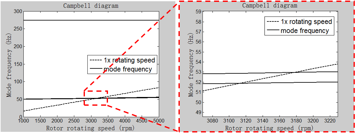
We can plot a Campbell diagram based on the results of the calculation. This is shown in the following figure. The first order forward critical speed of this sample rotor is approximately 3179 rpm.

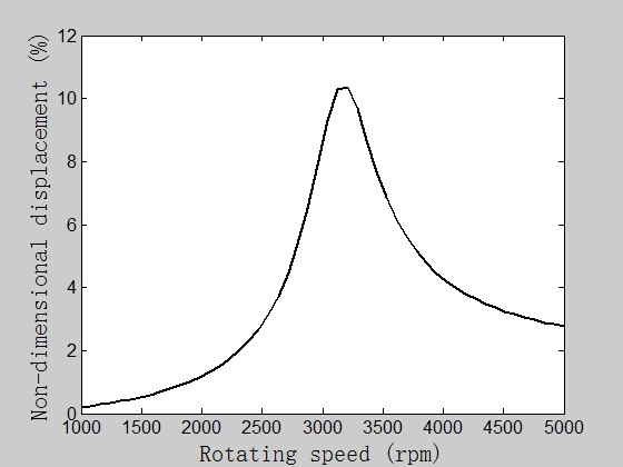
Likewise, the result of the unbalanced response analysis is illustrated in the following figure. Some unbalanced weight is applied on the left-most node of the rotordynamic Model. This node’s displacement amplitudes versus rotating speed are drawn as a curve. Those calculated amplitudes of displacement are non-dimensionalized by calculating the ratio of the amplitude to the width of the running clearance.