MATLAB: Generate Contour Image from CFD Results
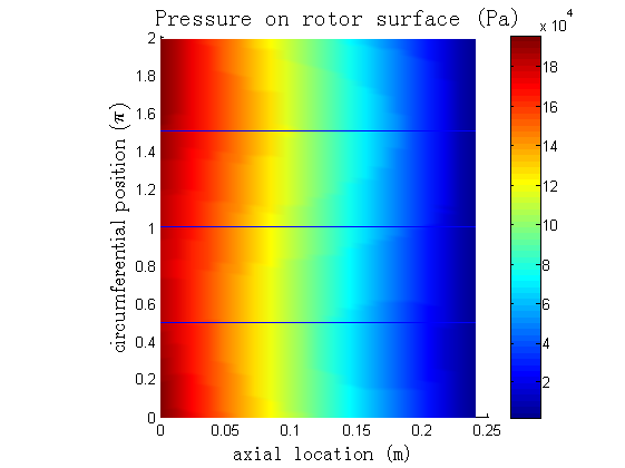
Since I have spent a lot of time studying the flow inside the running clearances in pumps, it becomes attractive if the calculated values on a rotor surface could be drawn as contours. So I decided to write a piece of Matlab code to do the job for me. The simulation data is exported from CFX-Post.
In order to generate the contour, I utilize the patch function of Matlab. For patch to work you have to tell it the topological structure of the grid and geometry. Thus, you have to export geometry data from CFX-Post. The geometry data holds the coordinate of each node and the connections among nodes for each element face. You feed these information into patch together with the calculated values, such as pressure, on all the nodes. Then patch will give you the contour image.
A sample contour looks like this ↓:
In fact, another Matlab function, griddata, seems more suitable for this purpose. I will look into that later.
The following list is the Matlab code. And associated m-files are listed here:
1
2
3
4
5
6
7
8
9
10
11
12
13
14
15
16
17
18
19
20
21
22
23
24
25
26
27
28
29
30
31
32
33
34
35
36
37
38
39
40
41
42
43
44
45
46
47
48
49
50
51
52
53
54
55
56
57
58
59
60
61
62
63
64
65
66
67
68
69
70
71
72
73
74
75
76
77
78
79
80
81
82
83
84
85
86
87
88
89
90
91
92
93
94
95
96
97
98
99
100
101
102
103
104
105
106
107
108
109
110
111
112
113
114
115
116
117
118
119
120
121
122
123
124
125
126
127
128
129
130
131
132
133
134
135
136
137
138
139
140
141
142
143
144
145
146
147
148
149
150
151
152
153
154
155
156
157
158
159
160
161
162
163
164
165
166
167
168
169
170
171
172
173
174
175
176
177
178
179
180
181
182
%
% File
% ====
%
% plot_pressure_rotor_surface.m
%
% Description
% ===========
%
% This script reads simulation data generated from CFX-Post. The data
% represents a pressure distribution on a rotor surface. The rotor is a
% cylinder. The user should export pressure data on the rotor surface
% together with the geometry information. The exported file could be a CSV
% file. The user can load this CSV file into Microsoft Excel. And then
% copy the columns of pressure and surface geometry data into two separate
% Matlab scripte files. One is get_node_p.m and the other is get_faces.m.
%
% This scripte reads back the two files and plot a pressure contour. The
% contour is on the unfold 2D x-theta plane, which is originaly a cylinder
% surface. The theta coordinates are calculated from the Cartesian
% coordinates of the surface nodes. Then, the issue of 0/2pi is properly
% handled.
%
% Author
% ======
%
% Yaoyu Hu <huyaoyu@sjtu.edu.cn>
%
% Date
% ====
%
% Created: 2016-10-14
%

% ====================== Preparation. ====================

% Clear the working space.
clear;
close all;
clc;

% Set searching directory.
restoredefaultpath;

% Constants.
NUM_NODES_PER_FACE = 4;
ONE_SEC_PI         = pi / 2;
TWO_PI             = 2 * pi;
THREE_SEC_PI       = 1.5 * pi;
THETA_LEN          = 2*pi/100 * 2;

% ========= Reload the node, presure and faces data. =========

% Load from prepared matlab file.
get_node_p;
get_faces;

% Re-arange the data.
node_x = node_P(:,1); % node_P is from get_node_p.
node_y = node_P(:,2);
node_z = node_P(:,3);
node_p = node_P(:,4);

maxP = max(node_p);
minP = min(node_p);
maxX = max(node_x);
minX = min(node_x);

clear node_P;
x = node_x;
clear node_x;

theta = get_angle(node_y, node_z);
clear node_y;
clear node_z;

faces = faces + 1; % faces is from get_faces.

% ============== Handle the 0/2pi issue. =============

[nFaces] = size(faces, 1);

nChanged      = 0;
idxBuffer     = [];
idxZeroBuffer = [];
rowBuffer     = [];

for I = 1:1:nFaces
    % Get the index
    idx = faces(I, :);

    % Get the angles.
    a = theta(idx);

    % Check.
    idxZero  = (abs(a) < ONE_SEC_PI);
    idxFirst = (abs(a) < THETA_LEN );
    idxBig   = (a > THREE_SEC_PI);

    sIdxZero  = sum(idxZero);
    sIdxFirst = sum(idxFirst);
    sIdxBig   = sum(idxBig);

    if ( sIdxZero >0 && sIdxBig > 0 && sIdxBig < 4 && sIdxZero + sIdxBig == 4)

        idxBuffer     = [idxBuffer;idx];
        idxZeroBuffer = [idxZeroBuffer;idxZero'];
        rowBuffer     = [rowBuffer;I];

        fprintf('I = %d, a = [ %e, %e, %e, %e]\n', I, a(1), a(2), a(3), a(4));
        nChanged = nChanged + 1;
    end
end % I

fprintf('nChanged = %d\n', nChanged);

for I = 1:1:nChanged
    row = rowBuffer(I,1);

    faces(row, :) = faces(1, :);
end % I

vertices = [x, theta / pi];

% ================ Check maximum face area. ========================

maxFaceArea = 0;
maxFaceIdx  = 0;

for I = 1:1:nFaces
    idx      = faces(I, :);
    faceX    = x(idx);
    faceT    = theta(idx);
    maxFaceX = max(faceX);
    minFaceX = min(faceX);
    maxFaceT = max(faceT);
    minFaceT = min(faceT);
    areaFace = ( maxFaceX - minFaceX ) * (maxFaceT - minFaceT);

    if ( areaFace > maxFaceArea )
        maxFaceArea = areaFace;
        maxFaceIdx  = I;
    end
end % I

fprintf('maxFaceArea = %e,idx = %d\n', maxFaceArea, maxFaceIdx);

% ==================== Patch plot. ======================

% Create a new figure.
h = figure;

% Patch.
p = patch('Faces', faces, 'Vertices', vertices);
set(gca, 'CLim', [minP, maxP]);
set(p,...
    'FaceColor', 'interp',...
    'FaceVertexCData', node_p,...
    'CDataMapping', 'scaled',...
    'EdgeColor', 'flat',...
    'LineStyle', 'none');
colorbar;

% Plot three horizontal lines to indicate 0.5pi, pi and 1.5pi
hold on;

plot([ minX,maxX],[0.5, 0.5]);
plot([ minX,maxX],[1.0, 1.0]);
plot([ minX,maxX],[1.5, 1.5]);

hold off;

% Set the labels and title of the patch plot.
xlabel('axial location (m)',...
    'FontSize', 14,...
    'FontName', 'Time New Rome');
ylabel('circumferential position ($ \pi $)',...
    'Interpreter', 'Latex',...
    'FontSize', 14);
title('Pressure on rotor surface (Pa)',...
    'FontSize', 16,...
    'FontName', 'Time New Rome');